Initial push
Hello! And welcome to this new blog post series, where I will be writing about technical matters that I find interesting.
In this kick-off article, I want to introduce the latest re-incarnation of my UAV simulator, last_letter. It’s a pet project that I’ve been carrying with me since 2013 and it has gone through many forms. It served me well during my PhD years and got a second life in my previous employment but for the most part it has been bit-rotting. I have spent the last two months reviving it and making it once again compatible with ArduPilot.
It consists of a C++ core, meant to offer very high update rates and cheap timesteps, and a set of Python bindings around it, to enable more freeform exploration of its models.
It’s not quite polished yet. I will keep it in v2.100+ until I’m happy with its API and then I’ll release a v3. But it can already offer an effective playground.
Today, we’ll do a short exploration of the thruster models that are offered by last_letter.
import last_letter as ll

thruster_simple = ll.propulsion.ThrusterSimple("simple")
thruster_beard = ll.propulsion.EngBeard("beard")
thruster_electric = ll.propulsion.ElectricEng("electric")
thruster_electric2 = ll.propulsion.ElectricEng2("electric2")
thruster_speed_control = ll.propulsion.EngOmegaControl("speed_control")
thruster_ice = ll.propulsion.PistonEng("ice")
ThrusterSimple is what its name says: It generates thrust and torque proportional to its input:
EngBeard is a simple model that incorporates pitch speed, taken from the excellent “Beard, R. W., & McLain, T. W. (2012). Small Unmanned Aircraft: Theory and Practice. Princeton University Press”.
EngOmegaControl hosts a propeller model whose power consumption and thrust generation go through polynomials of the advance ratio.
The propeller’s speed is governed directly by the thruster input, like a speed-controlled ESC.
ElectricEng runs a standard electric model with \(KV\), \(R\) and \(I_0\) parameters and a propeller whose power and efficiency are governed by a polynomial of the advance ratio. ElectricEng2 is almost identical, except the thrust generation goes through an independent polynomial of the advance ratio, instead of multiplying the consumed power with the propeller efficiency.
PistonEng is similar to ElectricEng, but instead of an electric motor it uses a motor whose power production is governed by a polynomial of the motor speed, akin to an internal combustion engine (ICE).
Let’s group those thrusters together and initialize them. This is necessary for them to read their parameters and instantiate the necessary submodels.
thrusters = [
    thruster_simple,
    thruster_beard,
    thruster_electric,
    thruster_electric2,
    thruster_speed_control,
    thruster_ice
]
for thruster in thrusters:
    thruster.initialize()
We can still change most parameters “on-the-fly”, after the thruster has been instantiated.
thruster_ice.set_param("thrustMax", 1000)
thruster_ice.set_param("engInertia", 200e-6)
thruster_ice.update_parameters()
thruster_electric.set_param("thrustMax", 1000)
thruster_electric.set_param("RadPSLimits", [0.01, 10000])
thruster_electric.update_parameters()
thruster_electric2.set_param("thrustMax", 1000)
thruster_electric2.set_param("RadPSLimits", [0.01, 10000])
thruster_electric2.update_parameters()
last_letter offers logging of the thruster wrench and speed. The log is of .mcap type, which is popular in robotics applications.
Let’s run each thruster across the throttle input range, waiting a little bit in each step for the thruster output to “settle”. The thrusters are “static” here, in the sense that they’re being operated in still air.
dt = thruster_simple.get_param_double("world/deltaT")
ll.enable_logging("001_static.mcap")

# Sweep across the throttle range.
for thr_idx in range(100):
    # Run each thruster for 0.5 seconds to let it stabilize.
    for t_idx in range(int(0.5/dt)):
        # Step each thruster.
        for thruster in thrusters:
            # The thrusters expect their throttle signal at index 0 by default.
            input = ll.utils.uav.Inputs.from_array([thr_idx/100])
            thruster.set_input(input)
            thruster.calc_model()
        # Log its final performance.
    ll.log_frame(thr_idx)
ll.disable_logging()
We can open the log file with the excellent PlotJuggler log viewer.
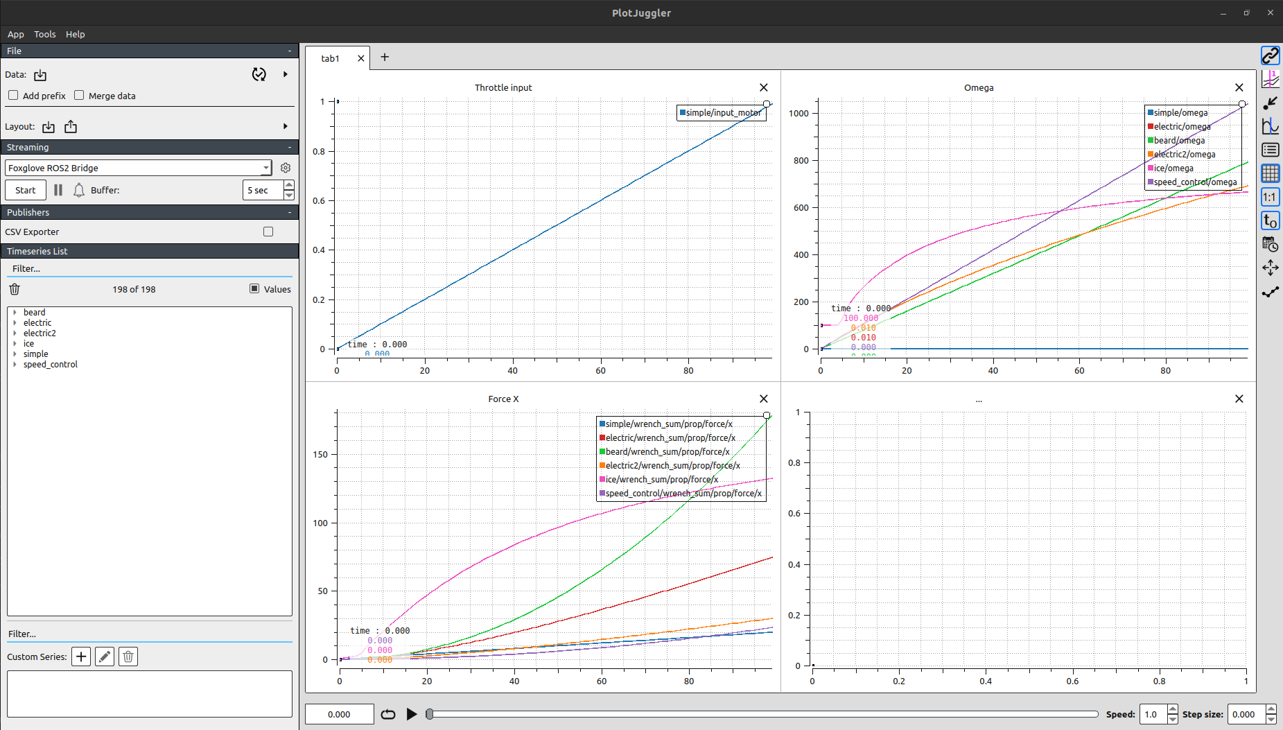
But we can also use last_letter utilities to convert the log file into a pandas frame or a .csv file, for more Python-friendly plotting.
import matplotlib.pyplot as plt

from last_letter.utils.log import load_log

FORCE_SERIES = "wrench_sum/prop/force/x"

# One channel per logged component, named after the component.
log = load_log("001_static.mcap")

fig, ax = plt.subplots(figsize=(9, 5))
for name, df in log.items():
    if FORCE_SERIES not in df.columns:
        continue
    # log_frame() was stamped with the throttle index, so the time axis of
    # every channel is the throttle command in percent.
    ax.plot(df.index, df[FORCE_SERIES], label=name)

ax.set_xlabel("throttle [%]")
ax.set_ylabel("thrust, body x [N]")
ax.set_title(FORCE_SERIES)
ax.grid(True)
ax.legend()
plt.show()
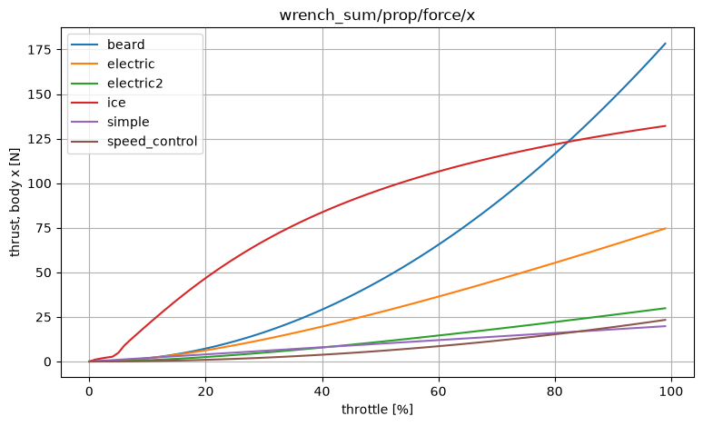
Thrust generation varies across these models. The Beard engine can produce up to 175N of thrust, whereas the Simple engine only 20N. Let’s try to scale them all to produce 100N max, in order to compare them more easilly.
The Simple engine can take a thrustMax parameter, whereas in the Beard engine we can scale the parameter for the propeller disk surface s_prop. In the Speed-controlled engine we can scale the propeller diameter in a similar fashion, through the parameter prop_diam. The Electric2 engine also offers a direct thrust scaler parameter propThrustMultiplier.
max_thrust = {name: df[FORCE_SERIES].max() for name, df in log.items() if FORCE_SERIES in df.columns}

thrust_target = 100
thruster_simple.set_param("thrustMax", thrust_target)
thruster_beard.set_param("s_prop", thruster_beard.get_param_double("s_prop")*thrust_target/max_thrust["beard"])
coeff = ( thrust_target/max_thrust["speed_control"] )**(1/4)
thruster_speed_control.set_param("prop_diam", thruster_speed_control.get_param_double("prop_diam")*coeff)
thruster_electric2.set_param("propThrustMultiplier", thrust_target/max_thrust["electric2"])
The rest of the engines don’t offer such a direct scaling parameter (room for improvement!) so we have to improvise.
We will pick a higher-cell pack for the Electric engine but choose a slightly smaller propeller. As for the ICE we’ll scale down the engine power parameters by 50%.
thruster_electric.set_param("prop_diam", 0.35)
thruster_electric.set_param("Cells", 8)

eng_poly = thruster_ice.get_param_vector("engPowerPoly/coeffs")
weak_eng_poly = [c*0.5 for c in eng_poly]
thruster_ice.set_param("engPowerPoly/coeffs", weak_eng_poly)
Don’t forget to call update_parameters() to load the changed parameters into the model.
for thruster in thrusters:
    thruster.update_parameters()
Let’s run the throttle sweep again.
ll.enable_logging("001_static_normalized.mcap")

for thr_idx in range(100):
    for t_idx in range(int(0.5/dt)):
        for thruster in thrusters:
            input = ll.utils.uav.Inputs.from_array([thr_idx/100])
            thruster.set_input(input)
            thruster.calc_model()
    ll.log_frame(thr_idx)
ll.disable_logging()

log = load_log("001_static_normalized.mcap")

fig, ax = plt.subplots(figsize=(9, 5))
for name, df in log.items():
    if FORCE_SERIES not in df.columns:
        continue
    ax.plot(df.index, df[FORCE_SERIES], label=name)

ax.set_xlabel("throttle [%]")
ax.set_ylabel("thrust, body x [N]")
ax.set_title(FORCE_SERIES)
ax.grid(True)
ax.legend()
plt.show()
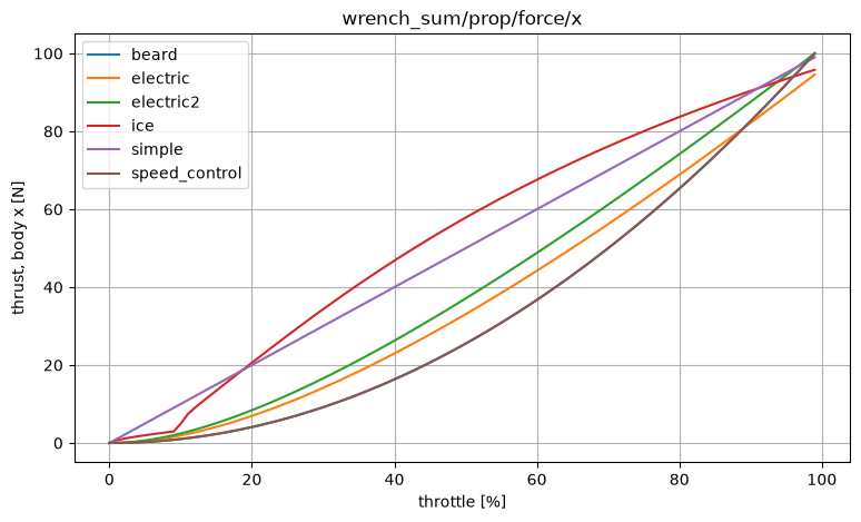
Nice! Now all the thrusters top out at roughly 100N. We can see that the Simple thruster has a completely linear response, whereas the others exhibit an exponential behaviour, common among electric thrusters. The ICE has an inverse curve, mostly due to the shape of its engine power polynomial.
Let’s also plot the thruster speed, in RPM:
import math

OMEGA_SERIES = "omega"

fig, ax = plt.subplots(figsize=(9, 5))
for name, df in log.items():
    if OMEGA_SERIES not in df.columns:
        continue
    ax.plot(df.index, df[OMEGA_SERIES]/(2*math.pi)*60, label=name)

ax.set_xlabel("throttle [%]")
ax.set_ylabel("propeller speed [RPM]")
ax.set_title(OMEGA_SERIES)
ax.grid(True)
ax.legend()
plt.show()
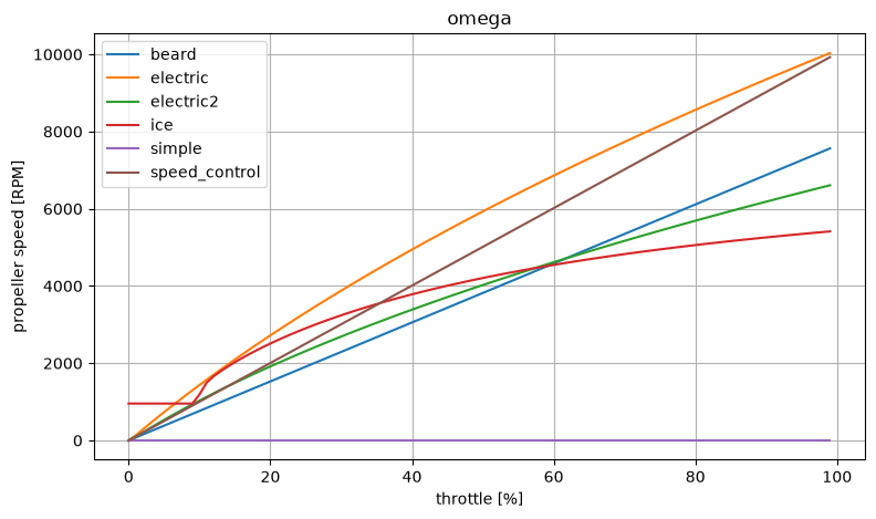
The Simple thruster has no notion of a rotating shaft, hence its speed is fixed at 0. The Speed-controlled thruster has a linear response, as expected. The Beard engine works the same.
The two electric engines have different speed curves, since the Electric motor runs on higher voltage and also the two propellers with different diameters load their respective motors differently.
The ICE will idle at ~950RPM until the throttle catches up with it.
You might have noticed that earlier I lowered the inertia of the internal combustion engine model. I did this because it was interfering with the experiment: It was taking too long to ramp up to a stable speed level.
Let’s spawn a fresh engine and see how long it actually takes to reach a stable speed.
thruster_ice_2 = ll.propulsion.PistonEng("ice_2")
thruster_ice_2.initialize()
thruster_ice.set_param("thrustMax", 1000)
eng_poly = thruster_ice_2.get_param_vector("engPowerPoly/coeffs")
weak_eng_poly = [c*0.5 for c in eng_poly]
thruster_ice_2.set_param("engPowerPoly/coeffs", weak_eng_poly)
thruster_ice_2.update_parameters()

ll.enable_logging("001_ice.mcap")


# Spend a little time on zero throttle.
input = ll.utils.uav.Inputs.from_array([0])
for t_idx in range (int(2/dt)):
    thruster_ice_2.set_input(input)
    thruster_ice_2.calc_model()
    ll.log_frame(t_idx*dt)

# Now raise throttle.
input = ll.utils.uav.Inputs.from_array([1])
for t_idx_2 in range (int(8/dt)):
    thruster_ice_2.set_input(input)
    thruster_ice_2.calc_model()
    ll.log_frame((t_idx + t_idx_2)*dt)

ll.disable_logging()

log = load_log("001_ice.mcap")

fig, ax = plt.subplots(figsize=(9, 5))
for name, df in log.items():
    if OMEGA_SERIES not in df.columns:
        continue
    ax.plot(df.index, df[OMEGA_SERIES]/(2*math.pi)*60, label=name)

ax.set_xlabel("step [-]")
ax.set_ylabel("propeller speed [RPM]")
ax.set_title(OMEGA_SERIES)
ax.grid(True)
ax.legend()
plt.show()
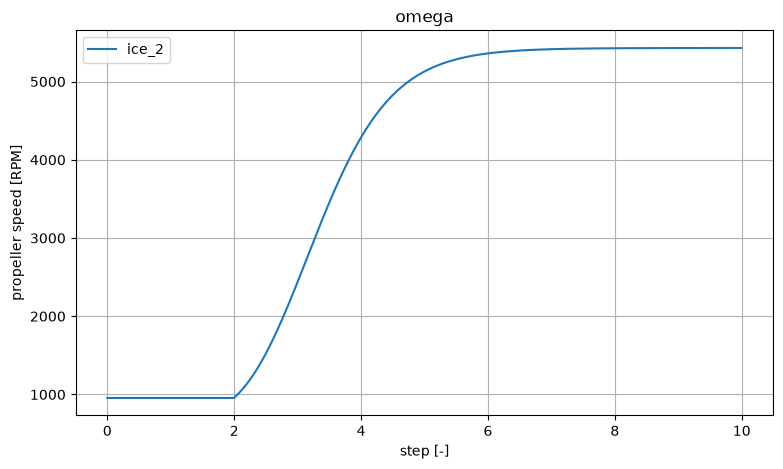
About 3s rise time. That’s a little on the slow side for an engine of that size, so the default model might need some tweaking. But that’s what parameters are there for.
Now let’s see how incoming air affects the thrust generation. In real life as the freestream air rushes faster towards a propeller (e.g. when an airplane flies) the propeller will “unload”, spin faster and produce less thrust, compared to how it runs on the ground.
We’ll update the EnvironmentData of the Thruster parent class, the Component and ramp up the wind along its longitudinal axis, from 0 to 10m/s.
environment = ll.environment.EnvironmentData()
state = ll.utils.uav.UavState()

for thruster in thrusters:
    thruster.update_local_state(state, environment)
    thruster.update_parameters()
ll.enable_logging("001_wind.mcap")

for wind_idx in range(11):
    environment.wind = [-wind_idx, 0, 0]
    for t_idx in range(int(0.5/dt)):
        for thruster in thrusters:
            thruster.update_local_state(state, environment)
            input = ll.utils.uav.Inputs.from_array([1.0])
            thruster.set_input(input)
            thruster.calc_model()
    ll.log_frame(wind_idx)
ll.disable_logging()

log = load_log("001_wind.mcap")

fig, ax = plt.subplots(figsize=(9, 5))
for name, df in log.items():
    if FORCE_SERIES not in df.columns:
        continue
    ax.plot(df.index, df[FORCE_SERIES], label=name)

ax.set_xlabel("headwind [m/s]")
ax.set_ylabel("thrust, body x [N]")
ax.set_title(FORCE_SERIES)
ax.grid(True)
ax.legend()
plt.show()

fig, ax = plt.subplots(figsize=(9, 5))
for name, df in log.items():
    if OMEGA_SERIES not in df.columns:
        continue
    ax.plot(df.index, df[OMEGA_SERIES]/(2*math.pi)*60, label=name)

ax.set_xlabel("throttle [%]")
ax.set_ylabel("propeller speed [RPM]")
ax.set_title(OMEGA_SERIES)
ax.grid(True)
ax.legend()
plt.show()
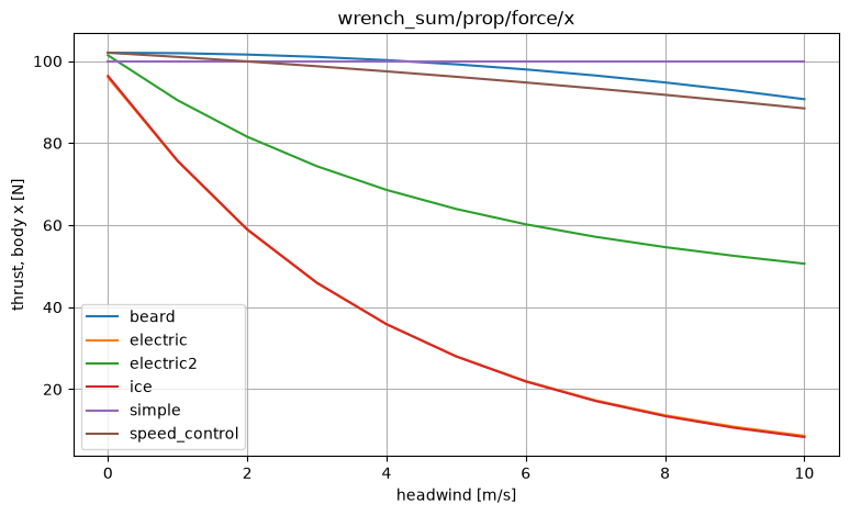
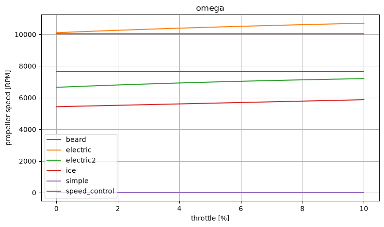
We see that all the thrusters that model a propeller with power polynomials of advance ratio (Electric, Electric2 and ICE) respond to the increasing headwind: the RPMs increase.
For these propellers, as well as the Beard and Speed-controlled engine, the generated thrust drops as headwind increases. For some it’s quite a bit more than I would expect, which probably means that our model parameters could use some tweaking, or at least grounding to real data.
Now let’s go back to our propeller collection and apply some wind coming from the side, along the propeller plane. We’ll do a throttle sweep under 10m/s sidewind.
environment.wind = [0, 10, 0]

for thruster in thrusters:
    thruster.update_local_state(state, environment)
    thruster.update_parameters()
ll.enable_logging("001_sidewind.mcap")

for thr_idx in range(100):
    for t_idx in range(int(0.5/dt)):
        for thruster in thrusters:
            input = ll.utils.uav.Inputs.from_array([thr_idx/100])
            thruster.set_input(input)
            thruster.calc_model()
    ll.log_frame(thr_idx)
ll.disable_logging()

log = load_log("001_sidewind.mcap")

SIDEFORCE_SERIES = "wrench_sum/prop/force/y"
fig, ax = plt.subplots(figsize=(9, 5))
for name, df in log.items():
    if SIDEFORCE_SERIES not in df.columns:
        continue
    ax.plot(df.index, df[SIDEFORCE_SERIES], label=name)

ax.set_xlabel("throttle [%]")
ax.set_ylabel("sideforce, body x [N]")
ax.set_title(SIDEFORCE_SERIES)
ax.grid(True)
ax.legend()
plt.show()
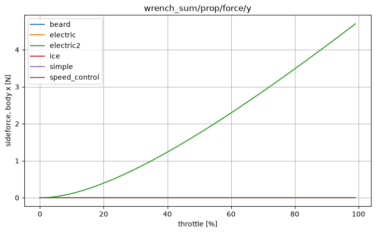
Only the Electric2 thruster models drag due to sidewind, in the form of momentum drag. The drag is proportional to the thrust and the sidewind.
\[F_y = -F_x V_{w,y} k_D\]That’s about enough for this article. All of these thruster models are available to compose aircraft in last_letter. Simpler ones are good for extracting arithmetic models and designing controllers around them, or simply removing complexity during experimentation on another part of the flight physics. Whereas more complex ones are useful for validation runs against a simulator that is as realistic as possible.
If you want to reproduce this exploration or modify it, you can download all the source files from here. last_letter is available from pypi, but you will have to build it locally. See what prerequisites you will need to do a Python build here.
It is strongly recommended you use the excellent uv toolchain to manage your installation.
Cheers!